VizCraft: A Multi-Dimensional Visualization Tool for Aircraft Design
My Master's thesis at Virginia Tech
Chapter 1Introduction
Scientists and engineers in many application domains commonly use modeling and simulation codes developed in-house that have poor documentation and a poor user interface. The code is often tied to a particular computing environment, and typically only the developers of the code can make effective use of it, reducing the productivity of many research groups. The recently proposed concept of problem solving environment (PSE) promises to provide scientists and engineers with integrated environments for problem solving in the scientific domain, increasing their productivity by allowing them to focus on the problem at hand rather than on general computation issues.
1.1 What is a PSE?
A PSE is a system that provides a complete, usable, and integrated set of high level facilities for solving problems in a specific domain [34, 44]. PSEs allow users to define and modify problems, choose solution strategies, interact with and manage appropriate hardware and software resources, visualize and analyze results, and record and coordinate extended problem solving tasks. In complex problem domains, a PSE may provide intelligent and expert assistance in selecting solution strategies, e.g., algorithms, software components, hardware resources, data, etc. Perhaps most significantly, users communicate with a PSE in the language of the problem, not in the language of a particular operating system, programming language, or network protocol. Expert knowledge of the underlying hardware or software is not required. Experience in dealing with large-scale engineering design and analysis problems has indicated the critical need for PSEs with four distinguishing characteristics: (1) facilitate the integration of diverse codes, (2) support human collaboration, (3) support the transparent use of distributed resources, and (4) provide advisory support to the user. In principle, PSEs can solve simple or complex problems, support both rapid prototyping and detailed analysis, and can be used both in introductory education and at the frontiers of science.
1.2 Problem Statement
Due to recent advances in computing facilities, visualization has taken up an important role in computational science and engineering, allowing scientists to gain an understanding of their data that was not previously possible. However, due to lack of integration among the various software modules, the visualization process is usually separate from the computation process that generates the data. This thesis describes two PSEs named VizCraft and WBCSim whose goal is to provide an environment in which visualization and computation are combined. The designer is encouraged to think in terms of the overall task of solving a problem, not simply using the visualization to view the results of the computation [14].
VizCraft is intended for aircraft designers working on the design of a High Speed Civil Transport (HSCT) [15, 46, 47, 68]. It has been developed in collaboration with the Multidisciplinary Analysis and Design (MAD) Center for Advanced Vehicles at Virginia Polytechnic Institute and State University. VizCraft provides a graphical user interface to command-line driven codes for design of the HSCT, besides providing components for visualizing the results of the computation. WBCSim is intended for wood scientists conducting research on wood-based composite (WBC) materials. It integrates FORTRAN 77-based simulation codes with a graphical, Web-based user interface, an optimization tool, and a visualization tool. WBCSim has been developed in collaboration with the Wood Science and Forest Products Department at Virginia Polytechnic Institute and State University.
1.3 Organization of Thesis
This thesis is organized as follows. Chapter 2 reviews numerous existing and emerging technologies that are related to the work presented in this thesis. We begin by discussing PSEs for the most common application areas, and then continue to discuss various other application domains that have been addressed by PSEs in the past. Chapter 3 discusses VizCraft, a PSE that provides an integrated environment for aircraft designers working with multidimensional design spaces. The design problem currently being faced by aircraft designers, some approaches that have been taken in the past towards solving it, and how VizCraft provides a unique approach in helping the designer visualize the problem, are presented. In Chapter 4 we discuss another PSE called WBCSim that provides a Web-based framework for wood scientists conducting research on wood-based composite materials. It integrates legacy simulation codes with a graphical front end, an optimization tool, and a visualization tool. Finally, Chapter 5 draws conclusions from the work described in previous chapters and discusses possibilities for future development.
Chapter 2
Related Work
A number of PSEs have been developed in the past for various application domains, and much of the design of our PSEs builds on ideas taken from them. PSE work consists of both the development of problem-specific PSEs and the development of general tools for building PSEs. Broader issues such as (1) developing a model or architecture for PSEs, (2) leveraging the Web, (3) supporting distributed, collaborative problem solving, and (4) providing software infrastructure ("middleware") are also being addressed.
2.1 PSEs for Partial Differential Equations
Partial differential equations (PDEs) are at the foundation of much of computational science. They can be used to model a variety of complex physical phenomena such as fluid flow, heat transfer, nuclear and chemical reactions, and population dynamics. Since it is generally impossible to obtain closed-form analytical solutions to these equations, their numerical solution plays an important role in our understanding of such physical phenomena. As a result, a vast amount of software has been developed for the numerical solution of PDEs, and it is not uncommon to see PSEs developed to address this problem. An early example is ELLPACK [12], a portable FORTRAN 77 system for solving two- and three-dimensional elliptic PDEs. Its strengths include a high-level language which allows users to define problems and solution strategies in a natural way (with little coding), and a relatively open architecture which allows expert users to contribute new problem solving modules. This allows expert users to iteratively solve nonlinear problems, time-dependent problems, and systems of equations. ELLPACK is suited for applications such as education, solving small prototype problems, and evaluating performance of software modules. Its large library of problem-solving modules allows users to easily experiment with a variety of numerical methods and assess their performance. ELLPACK's descendants include Interactive ELLPACK [26], which adds a graphical user interface and allows greater user interaction, and Parallel ELLPACK (PELL-PACK) [45], which includes a more sophisticated and portable user interface, incorporates a wider array of solvers, and can take advantage of multiprocessing. PELLPACK also includes an expert or "recommender" component named PYTHIA [58, 94] to automate the decision-making process and provide a high level abstraction to the user. Given a prescribed accuracy and solution time bound, PYTHIA attempts to match the characteristics of the given problem with those of some previously determined PDE problems to predict the appropriate method for solving a given problem. Moore at al. [75] describe a strategy for the automatic solution of PDEs at a different level. They are concerned with the problem of automatically determining a geometry discretization that leads to a solution guaranteed to be within a prescribed accuracy.
DEQSOL [89] solves linear elliptic problems on fairly general two- and three-dimensional domains with general linear boundary conditions. The development of DEQSOL has been driven by the desire to solve PDE systems resulting from relatively complex mathematical models such as in fluid mechanics or problems with material interfaces. The expression of solution of nonlinear problems, time-dependent problems, and systems of equations is more naturally achieved in DEQSOL than in ELLPACK. Another system that provides a high level, problem-oriented environment for PDE-solving is SciNapse [1], a code-generation system that transforms high-level descriptions of PDE problems into customized C or FORTRAN code, in an effort to eliminate the need for programming by hand. Other PSEs in the PDE problem domain include PDEase2D [95] and PDESOL [85].
2.2 PSEs for Multidisciplinary Design Optimization
In the past, a number of PSEs for MDO applications have been developed that provide frameworks for integrating analysis codes with optimization methods in a flexible manner, besides providing GUIs for reviewing the results of an optimization process. Framework for Inter-Disciplinary Optimization (FIDO) [96] demonstrates distributed and parallel execution of MDO applications using HSCT as its example. Increasingly complex models of the HSCT have been implemented in FIDO. Besides optimization, FIDO provides the ability to modify input parameters while the application is executing. iSIGHT [28, 88] provides a generic shell environment for supporting multidisciplinary optimization. A key feature of iSIGHT is its ability to combine numeric, exploratory, and heuristic methods during optimization. ISIGHT has been used to implement an HSCT application as well. LMS Optimus [42] allows users to set up a problem, select from a number of predefined methods to be used with the problem, and analyze the results. Capabilities include nonlinear optimization, design of experiments, and response surface methodologies. The DAKOTA iterator toolkit [27] provides a flexible, object-oriented, and extensible PSE for a variety of optimization methods including genetic algorithms. Besides optimization, methods are included for uncertainty quantification, parameter estimation, and sensitivity analysis. Lacking are integrated visualization, collaboration support, experiment management and archiving, and support for modifying the underlying simulation models. DAKOTA provides support for legacy code, high level component composition, and parallel computing. DAKOTA is capable of executing on a single processor as well as on a multiprocessor with message passing.
Messac et al. [71, 72] have developed PhysPro, a MATLAB-based application for visualizing the optimization process in real time using the physical programming paradigm. Among other visualization techniques, they use parallel coordinates to visualize the design metrics of the optimization process. The Visual Computing Environment (VCE) [61] provides a coupling between various ow analysis codes involved in multidisciplinary analysis codes at several levels of fidelity. Kingsley et al. [62] describe Multi-Disciplinary Computing Environment (MDICE), another PSE that provides users with a visual representation of the simulations being performed. It provides a distributed, object-oriented environment where many computer programs operate concurrently and cooperatively to solve a set of engineering problems. Several other MDO frameworks include Access Manager [81], NPSS [29],MIDAS [36], IMAGE [43], and AML [100]. The reader is referred to [84] for a more detailed examination of PSEs for MDO applications.
2.3 PSEs for Other Application Areas
PSEs are being built for a number of other scientific domains as well. For example, Parker et al. [77, 56, 76] describe SCIRun, a PSE that allows users to interactively compose, execute, and control a large-scale computer simulation by visually "steering" a data flow network model. SCIRun supports parallel computing and output visualization very well, but has no mechanisms for experiment managing and archiving, optimization, real-time collaboration, or modifying the simulation models themselves. Bramley et al. [13, 35] have developed Linear System Analyzer, a component-based PSE, for manipulating and solving large-scale sparse linear systems of equations. The components can be instantiated and run on remote systems and implemented in any mixture of languages. Users can then wire together these components in much the same way a design engineer wires together integrated circuits to build an application. Dabdub et al. [23, 22] have built an airshed PSE for modeling air pollution in urban areas. It provides a graphical user interface to a FORTRAN-based numerical solution model that takes into account many factors affecting air quality, like geography, weather patterns, sources of pollution, etc. The WISE environment [65] lets researchers link models of ecosystems from various sub disciplines.
The Information Power Grid (IPG) [9] being envisioned by NASA and the national laboratories is a completely general, all-encompassing PSE. While a few of the requisite technologies are in place (e.g., Globus [32] for distributed resource management, and PETSc [8, 41] for a scientific software library), it is unclear how the remaining components can be built and integrated. IPG is closer to a vision or goal than a working prototype. The law of conservation at work here seems to be that the power and level of integration of a PSE is directly proportional to the specificity of the problems being addressed by the PSE. Often, simulations used by computational scientists require access to significant computing resources, such as a parallel supercomputer or an "information grid" of computing resources. In such cases, the PSE should integrate a computing resource management subsystem such as Globus [32, 33] or Legion [66, 40].
An important goal of PSE researchers is to define a generic architecture for PSEs and to develop middleware (typically object-oriented) to facilitate the construction and tailoring of problem-specific PSEs [34]. This emphasis, along with work in Web-based, distributed, and collaborative PSEs, characterizes much of the current research in PSEs. For example, in [17] the authors describe PDELab, a multilayered, object-oriented framework for creating highlevel PSEs. PDELab supports PDESpec, a PDE specification language that allows usersto specify a PDE problem in terms of PDE objects and the relationships and interactions between them. Parallel Application WorkSpace (PAWS) [74] is a CORBA-based, object-oriented server for connecting parallel programs and objects. Other researchers investigating object-oriented frameworks for PSE-building include Gannon et al. [35], Balay et al. [7], and Long and Van Straalen [67].
2.4 Web-based PSEs
With the rise of the Web, PSEs are now beginning to support distributed problem solving frameworks. Web-based PSEs are ideal for facilitating collaboration among researchers and providing easy access to information. MDO is one of the application areas that can benefit greatly from this research. In [83, 82], Rogers et al. describe a Web-based framework for optimizing and controlling the execution sequence of design processes, and for visualizing the problem data. DARWIN [92] allows users to access data via the Web, while CGI scripts generate data for visualization purposes. Web-based PSEs have been developed for a number of other application areas as well. Regli [79] describes Internet enabled computer-aided design systems for engineering applications. Net PELLPACK [69], PELLPACK's Web-based counterpart, lets users solve PDE problems via Java applets. Other Web-based PSEs include NetSolve [16] and NEOS [21]. Current PSE related research projects that emphasize distributed collaboration include LabSpace [24], the Intelligent Synthesis Environment (ISE) [39], Habanero [18], Tango [10], Symphony [87], and Sieve [55]. One of the most impressive collaborative systems, in terms of capabilities and sophistication, is the CACTUS system [2] for the relativistic Einstein equations for astrophysics. CACTUS supports distributed computing, visualization, collaboration, experiment management, and model development. However, to adapt CACTUS to a different problem class is likely to be rather difficult, as the component tools are tailored to solving the astrophysics equations.
Chapter 3
VizCraft: A PSE for Configuration Design of a High Speed Civil Transport
This chapter describes VizCraft, a PSE that serves two purposes: (1) it provides a graphical user interface to HSCT design code developed at Virginia Polytechnic Institute and State University for the conceptual phase of aircraft design [15, 46, 47, 68], and (2) it provides components for visualizing the results of the computation. A detailed description of the working of our visualization tool is provided.
3.1 The HSCT Design Problem
The design of the HSCT is an active research topic at the Multidisciplinary Analysis and Design (MAD) Center for Advanced Vehicles at Virginia Polytechnic Institute and State University. The design problem is to minimize the take-off gross weight (TOGW) for a 250 passenger HSCT with a range of 5,500 nautical miles and a cruise speed of Mach 2.4. The simplified mission profile includes takeoff, supersonic cruise, and landing. For these efforts, a suite of low fidelity and medium fidelity analysis methods have been developed, which include several software packages obtained from NASA along with in-house software. A description of these tools is given by Dudley et al. [25].
We describe a PSE to aid aircraft designers during the conceptual design stage of the HSCT. Typically, the aircraft design process is comprised of three distinct phases: conceptual, preliminary, and detailed design. In the conceptual design stage, major design parameters for the final configuration are defined and set. The conceptual design phase models an aircraft with a set of values for significant parameters relating to the aircraft geometry, internal structure, systems, and mission. Examples of such parameters include the wing span, sweep, and thickness-to-chord ratios (t/c); the fuel and wing weights; the engine thrust; and the cruise altitude and climb rate, as shown in Table 3.1.
Individual designs can be (and are) viewed as points in a multidimensional design space [86]. The HSCT uses a design space with as many as 29 parameters. Two important features must be determined for any proposed design point: (1) it is feasible if it satisfies a series of constraints, and (2) it has a figure of merit determined by an objective function. The goal is then to find the feasible point with the smallest objective function value. In the multidisciplinary HSCT design problem, TOGW is chosen as the objective function. TOGW is a nonlinear, implicit function of the 29 design variables that define the HSCT configuration and mission. Using TOGW as the objective function provides a measure of quality with respect to a number of important aspects. The components of TOGW reflect the performance of the optimization. The fuel weight is determined primarily by the aerodynamic design, and the empty weight is set mainly by the structural design. The fuel weight is a measure of the operation cost, and the empty weight is an indicator of acquisition cost. In this way, TOGW is a good measure of the aerodynamic performance, structural efficiency, and economic feasibility of the aircraft [63].
The HSCT design uses 68 nonlinear inequality constraints. These are organized into two groups: geometric constraints versus aerodynamic/performance constraints, as shown in Table 3.2. Geometric constraints ensure feasible aircraft geometries. Examples include fuel volume limits and prevention of wing tip strike at landing with 5 degree roll. Aerodynamic constraints impose realistic performance and control capabilities. Examples include range requirements, landing angle-of-attack limits, and limits on the lift coefficient of the wing sections. Other aerodynamic constraints establish control of the aircraft during adverse flight conditions. These are complicated, nonlinear constraints that require aerodynamic forces and moments, stability and control derivatives, and center of gravity and inertia estimates [63].
In some respects, this is a classic optimization problem. The goal is to find that point which minimizes an objective function while meeting a series of constraints. However, this particular problem is difficult to solve for several reasons. First, evaluating an individual point to determine its value under the objective function and check if it satisfies the constraints is computationally expensive. A single aerodynamic analysis using a CFD code can take from 1-2 hour to several hours, depending on the grid used and flight condition considered. Second, the presence of numerical noise in the function values inhibits the use of many gradient-based optimization methods. This numerical noise may result in inaccurate calculation of gradients which in turn slows or prevents convergence during optimization, or it may promote convergence to spurious local optima [38, 6]. Third, the high dimensionality of the problem makes it impractical for many approaches that are often applied to difficult optimization problems. For example, genetic algorithms work poorly for this problem, since they require far too many function evaluations just to build a rich enough gene pool from which to begin the evolution. Fourth, the high dimensionality makes it difficult to even think about the problem spatially. Most people's intuitions about two- and three-dimensional space transfer poorly when considering behaviors in ten or more dimensions, or even in four dimensions.
| Number | Typical Value | Description |
| 1 | 181.48 | wing root chord, ft |
| 2 | 155.9 | leading edge break point, xft |
| 3 | 49.2 | leading edge break point, yft |
| 4 | 181.6 | trailing edge break point, xft |
| 5 | 64.2 | trailing edge break point, yft |
| 6 | 169.5 | leading edge wing tip, xft |
| 7 | 7.00 | wing tip chord, ft |
| 8 | 75.9 | wing semi-span, ft |
| 9 | 0.40 | chordwise location of maximum thickness |
| 10 | 3.69 | leading edge radius parameter |
| 11 | 2.58 | airfoil thickness-to-chord ratio at root, % |
| 12 | 2.16 | airfoil thickness-to-chord ratio at LE break, % |
| 13 | 1.80 | airfoil thickness-to-chord ratio at tip, % |
| 14 | 2.20 | fuselage axial restraint #1, xft |
| 15 | 1.06 | fuselage radius at axial restraint #1, rft |
| 16 | 12.20 | fuselage axial restraint #2, xft |
| 17 | 3.50 | fuselage radius at axial restraint #2, rft |
| 18 | 132.46 | fuselage axial restraint #3, xft |
| 19 | 5.34 | fuselage radius at axial restraint #3, rft |
| 20 | 248.67 | fuselage axial restraint #4, xft |
| 21 | 4.67 | fuselage radius at axial restraint #4, rft |
| 22 | 26.23 | location of inboard nacelle, ft |
| 23 | 32.39 | location of outboard nacelle, ft |
| 24 | 697.9 | vertical tail area, ft |
| 25 | 713.0 | horizontal tail area, ft |
| 26 | 39000 | thrust per engine, lb |
| 27 | 322617 | mission fuel, lb |
| 28 | 64794 | starting cruise/climb altitude, ft |
| 29 | 33.90 | supersonic cruise/climb rate, ft |
Table 3.1: Twenty-nine HSCT variables and their typical values
| Number | Geometric Constraints |
| 1 | fuel volume < = 50% wing volume |
| 2 | airfoil section spacing at >= 3.0ft |
| 3-20 | wing chord >= 7.0ft |
| 21 | leading edge break <= semi-span |
| 22 | trailing edge break <= semi-span |
| 23 | root chord t/c ratio >= 1.5% |
| 24 | leading edge break chord t/c ratio >= 1.5% |
| 25 | tip chord t/c ratio >= 1.5% |
| 26-30 | fuselage restraints |
| 31 | nacelle 1 outboard of fuselage |
| 32 | nacelle 1 inboard of nacelle 2 |
| 33 | nacelle 2 inboard of semi-span |
| 34 | range >= 5500 naut. mi. |
| 35 | lift coefficient (CL) at landing <= 1 |
| 36-53 | section CL at landing <= 2 |
| 54 | landing angle of attack <= 12degree |
| 55-58 | engine scrape at landing |
| 59 | wing tip scrape at landing |
| 60 | leading edge break scrape at landing |
| 61 | rudder detection <= 22.5 degree |
| 62 | bank angle at landing <= 5degree |
| 63 | tail detection at approach <= 22.5 degree |
| 64 | takeoff rotation to occur <= Vmin |
| 65 | engine-out limit with vertical tail |
| 66 | balanced field length <= 11000ft |
| 67-68 | mission segments: thrust available >= thrust required |
Table 3.2: Constraints for the 29 variable HSCT optimization problem
The region enclosed by the lower and upper bounds on the variables is termed the design space, the vertices of which determine a 29-dimensional hypercube. The high dimensionality of the problem makes visualization of the design space difficult, since most standard visualization techniques do not apply. In practice, we can only hope to ever evaluate a small fraction of the points in this design space. This is not only because evaluating a single point is expensive, but also because the number of points is impossibly large. Consider evaluating only the points that represent combinations for the extreme ends of the range in each parameter. In three dimensions, this would be equivalent to evaluating the eight corners of a cube. In 29 dimensions, 229 = 1/2 billion point evaluations would be required.
3.2 The Visualization Challenge
Given the difficulty and practical significance of the initial design problem, aircraft designers are searching both for new ways to find better design points, and for new insights into the nature of the problem itself. Visualization holds some promise for providing insights into the problem through the ability to provide new interpretations of available data. Visualization might also help, in conjunction with some form of organization for earlier point evaluations, to allow the designer to search through the design space in some meaningful way.
Thus, the challenge to the visualization community is to devise techniques that help aircraft designers during the conceptual design stage. The hope is that visualization can be used to let engineers apply their design expertise to the problem, and to guide the computation. Unfortunately, existing techniques for visualizing multidimensional spaces [11, 19, 30] do not apply to this problem.
Since the dimension of the problem is so large, any attempt to directly visualize the entire space through time series techniques, animation, use of color and transparency, sound, etc., cannot succeed. Of course, it may be of help to visualize relatively low-dimensional sections of the design space (a simple example of this approach is described in the next section).
Techniques for visualizing multidimensional spaces include parallel coordinates [49, 52] and a scatterplot matrix [11, 30]. Both essentially allow comparisons of (arbitrary) pairs of variables, and do not help with recognizing spatial relationships between points in the N-dimensional space. A disadvantage to using scatterplots is that too many plots are needed to obtain a comprehensive view of the relationships between variables in the design space. Various clustering methods have been proposed that attempt to map similarities in data records from a high dimensional space into a two- or three-dimensional space [99, 5]. Unfortunately, it is not clear what it means for design points to be "similar" aside from obvious measures such as similar objective function values, nor is it clear how this approach would provide insight to designers.
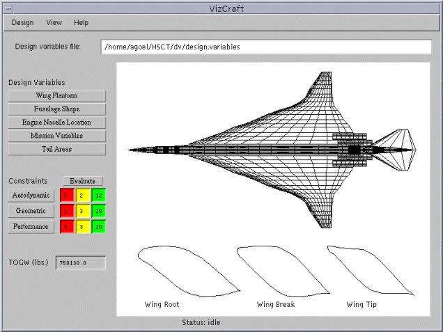
Figure 3.1: VizCraft design view window showing aircraft geometry and cross sections of the airfoil at the root, leading edge break, and tip of the wing. The panel on the left indicates the number of violated (red), active (yellow), and satisfied (green) constraints, and allows the user to modify values of design variables.
It is interesting to compare the aircraft design problem described here to other problems in multidimensional data analysis more frequently encountered. To illustrate this class of problems, consider locating a place to retire. There might typically be 10 or 20 variables to consider when evaluating possible retirement places, such as climate, population density, crime rate, etc. Data analysis for the retirement problem depends on building an objective function that attempts to assign values to each parameter on some linear scale and relative weights to the various parameters.
There are important differences in the two problems that affect their visualizations. In the retirement problem, for each variable, more (or less) of most parameters is absolutely better. There is effectively a fixed number of destinations, and there may not exist a point A differing from B only in one variable. In the aircraft design problem, all points in the parameter space are possible for consideration. However, one cannot simply choose the point that independently optimizes each parameter for two reasons. One reason is that the constraints supply an independent limitation on the values of various parameter combinations, so that improving one parameter independent of the others may violate some constraint. More important, however, is the fact that there is a nonlinear relationship between the parameters as they affect the objective function in the aircraft design problem. In particular, the objective function is non monotonic with respect to many of the design parameters.
3.3 First Efforts
Visualization techniques have already been applied to the aircraft design problem in two ways. First, a point in multidimensional space corresponds to an aircraft configuration. It is of use to the designer to be able to see an iconic representation of the airplane shape that corresponds to a given point, such as illustrated by Figure 3.1. The parametric representation is transferred to physical coordinates and stored in the Craidon geometry format [20] which serves as input to several of the analysis methods. The physical coordinates could as well be stored in any other suitable format, but in our HSCT design model, we use the Craidon geometry format. These physical points are then formatted as input to a plotting package.
The second use of visualization illustrates the power of even simple visualizations to provide insight into a difficult problem. Figure 3.2 (from [64] shows a triangular section of a two-dimensional slice through the multidimensional design space using Optimum 1, Optimum 2, and another sub optimal feasible point. The remaining points are created by linearly varying the design variables between all three points. This figure is somewhat misleading in that it is normally unusual to have gathered so much information about a particular region of the design space. The relatively large number of point evaluations were performed expressly to generate the image.
In Figure 3.2, the circles represent design points. Open circles represent feasible points while filled circles represent points that have violated some constraints. The value of the objective function is indicated by the shading. In this particular region of the design space, the objective function is relatively insensitive, resulting in a smooth "surface", because all three points selected have similar objective function values -- in the HSCT problem, numerical noise affects mostly the constraints. The lines on the plot represent the boundaries of four constraints. The lines are actually generated from interpolating the data achieved from the point evaluations -- there do not exist simple independent equations that can be used to discriminate large sets of points as satisfying or violating an individual constraint, except as gross approximations.
Designers need insight into the shape of the design space in which they work. Knowledge of the constraint boundaries and variation in objective function value can allow more informed selection of optimal designs.
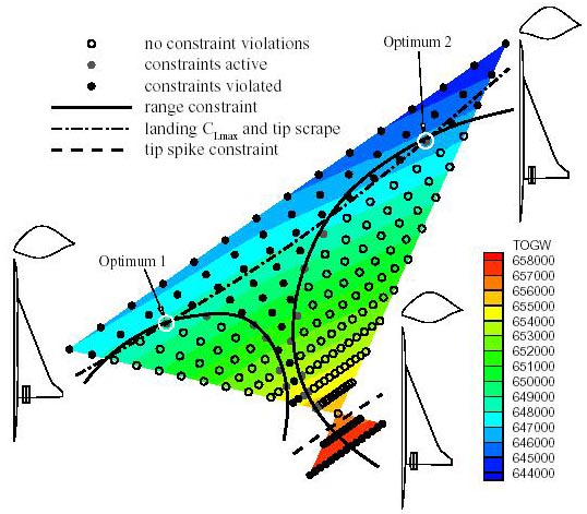
Figure 3.2: A two-dimensional slice through a multidimensional parameter space [64] using Optimum 1, Optimum 2, and another sub optimal feasible point. The circles on the plot represent design points, lines represent the boundaries of four constraints, and the shading indicates the value of the objective function.
The reason for developing this 2-D slice visualization was to gain some insight into the properties of the design space. The original motivation came from the results of an automated optimizer applied to the problem. It was known that the optimizer was sensitive to initial conditions, in that providing one starting point yielded a local optimum, while providing another starting point yielded another local optimum that was 2000 lbs lighter. Prior to creating the visualization, it was not recognized that the constraints break the design space into disjoint (at least in some hyper planes) regions of feasible points.
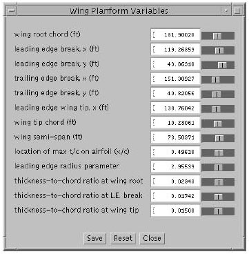
Figure 3.3: Input window for entering values of wing planform variables. Values of the variables must lie within a certain valid range indicated by the position of the slider thumbs.
This insight came as a result of the visualization. Knowing whether to accept (or reject) what the optimizer tells us is important. Optimizers can have trouble in high-dimensional, highly constrained problems. Using visualization in conjunction with optimization can provide understanding of the optimization process and trade-offs involved, but it also has the potential to provide guidance by an experienced engineer when the optimizer runs into trouble (such as when the gradient of the objective function is nearly perpendicular to a constraint boundary).
3.4 Design Point Visualization
In the absence of a better automated technique for solving the problem, aircraft designers would benefit from better visualization tools for helping select better designs. One approach might be a visualization system that helps better manage the information available. We have developed VizCraft, a pair of tools for visualizing HSCT designs. The first tool permits the user to quickly evaluate the quality of a given design with respect to its objective function, constraint violations, and graphical view. The second tool is an implementation of the parallel coordinates visualization [49, 52]. Its goal is to allow the user to effectively investigate a database of designs.
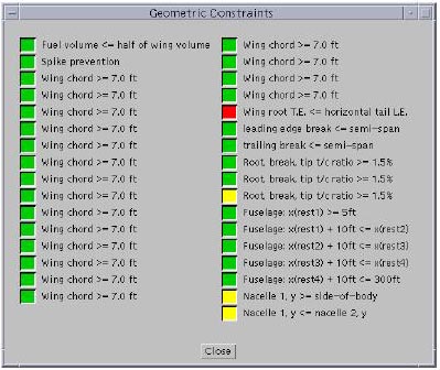
Figure 3.4: Geometric constraints for one design point. A red-colored box indicates a violated constraint, a yellow box indicates an active constraint, and a green box indicates a satisfied constraint.
VizCraft provides a menu-driven graphical user interface to the HSCT design code [68], a collection of C and FORTRAN routines that calculate the aircraft geometry in 3-D, the design constraint values, and the TOGW value, among other things. Java was chosen as the programming language for development because (1) users of VizCraft needed the ability to execute it from various UNIX platforms without concerning themselves with user interface library installation issues, and (2) implementing it in Java would give us the ability to later cast VizCraft as an applet and leverage the Web, an important design goal of VizCraft, especially of the parallel coodinates module (described in the next section).
Figure 3.1 shows VizCraft's main window with a display of the HSCT planform (a top view) for a sample design. Below the planform are displayed cross sections of the airfoil at the root, leading edge break, and tip of the wing, in that order. To make observation easier, the vertical dimension of the cross sections has been magnified. Prior to developing VizCraft, designers used Tecplot to display the HSCT planform, but we decided to write a conversion routine to integrate the planform into VizCraft. This had the advantage that users would not have to run a different application along with VizCraft to view the aircraft geometry. Integration allows engineers to shift easily between a visual representation of the design and points in design space. In addition to the static top view, we added a VRML [3] model of the HSCT planform, accessible from the menu bar. This provides the user with greater flexibility in manipulating the planform in 3-D, with ease of manipulation depending on the VRML browser used.
The vertical panel to the left of the planform in Figure 3.1 provides access to more information about the current design point. The design variables have been divided into five categories: wing planform, fuselage shape, engine nacelle location, mission variables, and tail areas. The constraints have been divided into geometric, aerodynamic, and performance constraints. Clicking on the "Wing Planform" button in the main window pops up the window shown in Figure 3.3. This window displays the wing parameters and the values currently assigned to them. The sliders on the right can be used to modify the values of the corresponding design variables. Each time the value of a design variable is modified, the HSCT planform is immediately updated to reflect the new geometry, and so is the value of TOGW on the vertical panel. Constraints for the current design point are not automatically evaluated after each change to an input parameter, however. Since constraint evaluation is time-consuming even for the low fidelity model we are using (taking approximately 10 seconds on a dual-processor DEC Alpha 4100 5/400 under typical user loads), VizCraft evaluates constraints only when the user explicitly requests it by clicking on the "Evaluate" button shown in Figure 3.1.
Once constraints are evaluated, the user is given feedback in various ways. The colored boxes shown in Figure 3.1 represent information about the number of constraints violated, active, and satisfied but inactive in each category of constraints. The red boxes indicate
the number of constraints of that category that are violated, the yellow boxes indicate the number of constraints that are "active", (i.e., close to a constraint boundary), and the green boxes indicate the number of constraints that are satisfied and inactive. Since all constraint values have been normalized to a common scale, it suffices to know that if the value of a constraint lies below
Clicking on the "Geometric" Constraints button pops up the window shown in Figure 3.4. This window lists the geometric constraints for the current design point, and a colored box next to each one indicates if it is violated (red), active (yellow), or inactive (green).
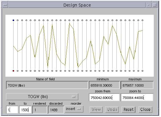
Figure 3.5: Parallel coordinates representation of one design point using 31 vertical lines. Each vertical line represents a design parameter. The first line from the left represents the TOGW (the objective function), the second line represents the HSCT range (a critical constraint value derived along with the TOGW for a given design), and the remaining 29 lines represent the design variables.
3.5 Parallel Coordinates
The tool described in the previous section provides a visualization of the aircraft that would be derived from a given design vector, and also provides a convenient view of constraint violations. However, it does not help designers with the more difficult task of understanding how a proposed design compares with other designs. This task is complicated by the high dimensionality of the design problem, and the resulting difficulty in visualizing or comprehending the multidimensional design space. Few visualization techniques provide an adequate visualization of high-dimensional spaces. Cartesian coordinates certainly do not provide an easy means of representing higher dimensional systems. Additionally, since all dimensions are equally important for the HSCT design, and since we do not know where in the design space lies the region of optimal design, we cannot afford to use techniques that suffer from data hiding. Data hiding can adversely affect the accuracy with which the design space is perceived.
One method of visualizing multiple dimensions, while retaining all the important mathematical information contained in the multidimensional space, is based on the concept of parallel coordinates. Parallel coordinates were proposed by Alfred Inselberg [48] as a new way to represent multidimensional information. Since the original proposal, much subsequent work has been accomplished, e.g., [49, 54], and parallel coordinates have been applied to a variety of multivariate problems including robotics, aerospace, management science, computational geometry, computer vision, conflict resolution in air traffic control, process control and instrumentation, power stability analysis, thermodynamic processes, differential equations, and statistics [51, 53].
A parallel coordinates visualization assigns one vertical axis to each visualization variable, and evenly spaces these axes horizontally, as shown in Figure 3.5. This is in contrast to the traditional Cartesian coordinates system where all axes are mutually perpendicular. By drawing the axes parallel to one another, one can represent points in much greater than three dimensions. In our application, potential visualization variables (equivalently, dimensions) include the design variables, the objective function value, and the constraint values. Each visualization variable is plotted on its own axis, and the values of the variables on adjacent axes are connected by straight lines, as shown in Figure 3.5. Thus, a point in an n-dimensional space becomes a polygonal line laid out across the n parallel axes with n - 1 line segments connecting the n data values. Many such data points (in Euclidean space) will map to many of these polygonal lines in a parallel coordinate representation. Viewed as a whole, these many lines might well exhibit coherent patterns which could be associated with inherent correlation of the data points involved. In this way, the search for relations among the design variables is transformed into a 2-D pattern recognition problem, and the design points become amenable to visualization.
One important aspect of this visualization scheme is that it provides opportunities for human pattern recognition: by using color to distinguish lines, and by supporting various forms of interaction with the parallel coordinates system, patterns can be picked up in the given database of design points. Given the upper and lower limits on each variable, the location of a polygonal line laid out across the n vertical axes gives some idea as to where that design point lies in the design space. The number of dimensions that can be visualized using this scheme is fairly large, limited only by the horizontal resolution of the screen. However, as the number of dimensions increases, the axes come closer to each other, making it more difficult to perceive patterns.
It is also important to note the flexibility of the parallel coordinates approach in that each coordinate can be individually scaled -- some may be linear with different bounds, while others may be logarithmic (although logarithmic scaling is currently not supported by VizCraft). While this prevents us from observing the exact relationships between various parameters, it may aid in identifying direct, inverse, and one-to-one relationships between the parameters.
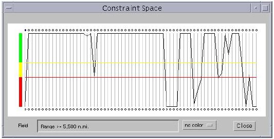
Figure 3.6: Parallel coordinates representation of 68 constraints for one design point. Horizontal lines split the vertical lines into three regions: satisfied, active, and violated. Any constraint falling below the red horizontal line is considered violated. This kind of a graphical representation avoids having to deal directly with numbers.
Scaling an individual parameter has another advantage in that it helps us in zooming into or zooming out of a subset of the region of design space represented, effectively brushing out or eliminating undesirable portions of the design space.
In Figure 3.5, 31 values are shown mapped onto 31 vertical axes. The first axis represents the TOGW, the second represents the HSCT range (a critical constraint value derived along with the TOGW for a given design), and the remaining 29 axes represent the 29 design variables. Placing the mouse cursor on one of the circles below the vertical lines will cause the "Name of field" text field to display a description of the corresponding visualization variable. The white text boxes indicate that the displayed range for the TOGW is from 750042.6 lbs ("zoom from" field) to 750064.44 lbs ("zoom to" field), whereas the absolute range for the TOGW is from 655918.3 lbs ("minimum" field) to 875657.1 lbs ("maximum" field). The absolute ranges for all the design variables are obtained automatically by locating their minimum and maximum values from the given database of points. Other details about the display controls will be explained as they become more relevant.
Figure 3.6 shows the parallel coordinates system for 68 constraints corresponding to the design point shown in Figure 3.5. All constraint values are normalized, with the range for violated, active, and inactive values being consistent across the constraints. All values above the yellow horizontal line indicate inactive constraints, all values between the yellow and red lines indicate active constraints, and all values below the red horizontal line indicate violated constraints.
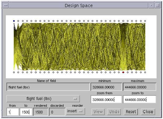
Figure 3.7: Parallel coordinates representation of 1500 design points selected uniformly from the entire design space. Each polygonal line (representing one design point) is assigned a color based on the value of a particular visualization parameter.
This kind of visualization is called physical programming-based visualization (PPV) [73] which calls for assigning ranges of differing degrees of desirability to each design metric. PPV has the following advantages: (1) it obviates the need for the designer to deal with numbers while assessing the "goodness" of a design metric, and (2) a quick glance at the screen conveys most of the information the designer needs in order to form a judgement of the current point(s). In this way, assessment of the design metrics requires minimum effort on the part of the designer. In Figure 3.6, by breaking up the range of constraint values into three regions, it becomes easy to graphically identify the inactive and violated constraints, and to what degree each constraint has been violated, without having to deal directly with numbers.
Representing just one design point in the parallel coordinates system may help the designer quickly view the level of constraint violations, but this is little better than the view provided by the single-point VizCraft tool. The real purpose of parallel coordinates in VizCraft is to allow the designer to browse a database of design points. We illustrate this process with a database of 1500 design points selected uniformly from the entire design space. When this database is rendered, it appears as shown in Figure 3.7. From this mass of data, one can use VizCraft's visualization controls to extract patterns. Each polygonal line (representing one design point) is assigned a color based on the value of a particular visualization parameter.
In Figure 3.7, the value used to determine the color is TOGW. Thus, as lines span across the vertical axes, one can identify those design points for which the TOGW is high or low. The design point with lowest value of TOGW is assigned a yellow color, the one with the highest value is assigned a black color, while the color for all the other design points is a linear interpolation between yellow and black. Since the design objective is to minimize the TOGW, the designer might initially be interested in lines rendered in yellow. However, the primary purpose of the parallel coordinates tool is to allow the user to investigate correlations between various visualization parameters, independent of the specific application context. For example, it may prove equally useful to the designer to discover that certain design variable ranges are associated with bad designs as it is to discover that other ranges are associated with good designs.
Looking at Figure 3.7, one can already see from the color gradation that the sixth axis from the right is directly related to the first axis. It so happens that the sixth axis from the right represents the weight of the flight fuel in lbs, which affects the TOGW directly. One can also observe that the second axis from the left is also mildly correlated to the TOGW and flight fuel. This axis represents the range of the aircraft in nautical miles, which must be directly proportional to the amount of fuel added. Even though these particular relationships are obvious (once the viewer has an understanding of the parameters involved), they give us a good start into understanding how to extract patterns from the data.
3.6 Visual Data Mining
A display of the full database such as shown in Figure 3.7, is typically too overwhelming to gain any real understanding of the data. The real strength of the parallel coordinates tool in VizCraft is the capability it provides for exploring the database. In this section we explain how the user can interact with the system "visual cues" [50] that will help in visualizing the data set in n-dimensional space. Looking at Figure 3.7, notice that there is a circle above each vertical axis, and that only the first one on the left is shaded. The shaded circle indicates the visualization variable that is currently "driving" the gradation of color across the parallel coordinates. For example, in Figure 3.7, TOGW is driving the color gradation. The user can select any visualization variable to drive the coloring by clicking inside the circle over the corresponding variable's axis. Clicking on the fifth circle we see that that variable happens to share a direct relationship with the seventh visualization variable (Figure 3.8). This shows that a clever selection of color drivers can help us extract patterns from the data set -- patterns which are otherwise hidden underneath the volume of data. Such patterns must exist in the data set, because 1500 points in 29 dimensions is a very sparse experimental design. A uniform sampling would contain at least as explained in Section 3.
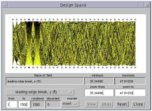
Figure 3.8: A clever selection of the "color driver" variable highlights a relationship between two visualization variables
The user's ability to recognize patterns in the parallel coordinates representation can be greatly affected by the sequence in which the axes are placed. For example, it is easier to perceive relationships between two adjacent axes than if the two axes are placed far apart. VizCraft allows the user to rearrange the axes. The user simply clicks on the circle above the axis to be moved and drags it to the new position. As an example, to insert the jth axis between the fifth and kth axes, the user must click on the circle located above or below the fifth vertical line, drag the mouse pointer and release it somewhere between the fifth and kth vertical lines, e.g., inserting the seventh axis before the sixth axis in Figure 3.8 results in Figure 3.9. It brings up clearly the one-to-one relationship shared by the fifth and seventh design variables. This rearrangement must be done with the reorder option set to "insert". If the reorder option is set to "swap", then one axis can be swapped with another by clicking and dragging one circle onto another. See [4] for a discussion on automating the process of initially arranging the axes to maximize similarities between adjacent axes.
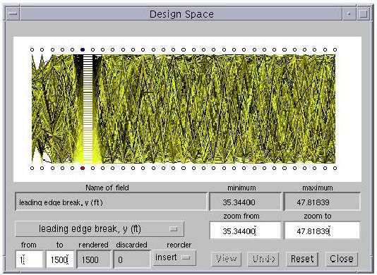
Figure 3.9: A clever rearrangement of the design variables brings up a one-to-one relationship between two variables in the data set.
While showing a large number of design points can be helpful in generating patterns that may be of interest to the researcher at a holistic level, individual design points cannot be distinguished when too many are displayed at once. To allow clear views of individual design points, the user may wish to select from this design space a sub region of interest, or a sub region that meets certain criteria. For example, the user may wish to eliminate all design points for which TOGW is greater than 700,000 lbs, or eliminate those points for which the range of the aircraft is less than 4,000 miles. The goal is to allow the user to gain some understanding of spatial relationships in n-space by selecting all data points that fall within a user defined set. This technique of graphically selecting or highlighting subsets of the data set is called "brushing" [93, 98].
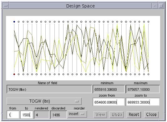
Figure 3.10: Result of brushing out design points lying outside a certain range of TOGW.
VizCraft makes it particularly easy to extract regions of interest from the design space. For example, to select a region for which TOGW lies within a certain range, the user can select the circle below the TOGW axis, and then enter the range in the "zoom from" and "zoom to" textboxes. This eliminates all design points for which the value of TOGW does not lie within this range. The axis for TOGW is recalibrated to this new scale, while all other axes retain their calibration. Alternatively, the user can click on any axis, drag the mouse pointer up or down, and release it to zoom into a region of interest. Figure 3.10 shows the result of zooming into a region of low TOGW. The text boxes at the bottom indicate that there are only four design points lying in the region of interest, and that the remaining 1,496 points have been discarded. Since we are interested in designs that yield low values for TOGW, we can now observe other design variables in this design subspace. Perhaps this will allow the designer to gain insight regarding what values of these variables, or what combinations of values of these variables, produced low values of TOGW.
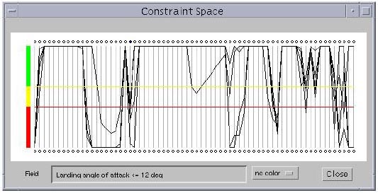
Figure 3.11: Constraints for the four design points shown in Figure 3.10. The "no color" option indicates that the polygonal lines representing all the design points are rendered in the default color (black in this case).
Figure 3.11 shows the set of constraints corresponding to Figure 3.10. VizCraft provides application-specific visualization options related to constraint violations. The "no color" option indicates that the polygonal lines representing all the design points are rendered in the default color. The "all" option indicates that the polygonal lines are colored using a rule that if any constraint is violated for a particular design point, that design point must be rendered in red. If all constraints are satisfied for a particular design point, that design point is rendered in green. In Figure 3.11 there is no design point that satisfies all constraints. A third option, the "selective" coloring option, assigns a color to each polygonal line on the rule that all points for which the selected constraint is violated are colored red, those points for which that constraint is active are colored yellow, and those points for which that constraint is satisfied are colored green. As in the case of design variables, the user can select any constraint to drive the coloration by clicking on the oval on top of the vertical line corresponding to that constraint. In Figure 3.12, coloring is being driven by the forty-second constraint from the left (i.e., No engine scrape at landing angle-of-attack). Out of the four cases displayed, this constraint is satisfied once, is active once, and is violated twice. This coloration scheme can give an idea of the troublesome constraints, ones that are usually violated. Unlike the other visualization variables, the constraint values lying beyond the range of the vertical lines are truncated. This becomes necessary to maintain the positions of constraint boundary lines, i.e., the horizontal red and yellow lines.
Finally, VizCraft gives the user an opportunity to click and highlight any one of the design points. To highlight a design point, the user must click at a point where a polygonal line intersects a vertical axis. Highlighting is done by assigning a bright color to the design point of interest. The highlighted point can also be viewed in its iconic representation in the main window (as in Figure 3.1) by clicking on the "View" button.
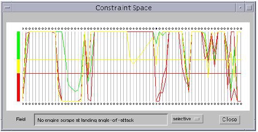
Figure 3.12: Constraints for the four design points shown in Figure 3.10, with selective coloring. The selective coloring option assigns a color to each polygonal line on the rule that all points for which the selected constraint is violated are colored red, those points for which that constraint is active are colored yellow, and those points for which that constraint is satisfied are colored green. Here, coloring is being driven by the forty-second constraint from the left (i.e., No engine scrape at landing angle-of-attack). Out of the four cases displayed, this constraint is satisfied once, is active once, and is violated twice.
By incorporating various forms of interaction into the parallel coordinates system, VizCraft provides a framework that allows the designer to visualize databases of HSCT designs. It allows the user to visually manipulate the design space while searching for patterns, and to eliminate portions of the design space from consideration by carefully selecting regions of interest. However, an intuitive feel for this application of parallel coordinates can only be realized with some practice, just as an intuitive feel for Cartesian representations is developed through usage and practice.
Chapter 4
WBCSim: A Prototype PSE for Wood-Based Composites Simulations
This chapter describes a computing environment named WBCSim that is intended to increase the productivity of wood scientists conducting research on wood-based composite (WBC) materials. WBCSim integrates FORTRAN 77-based simulation codes with a graphical, Web-based user interface, an optimization tool, and a visualization tool.
The objective of WBCSim is twofold: (1) to increase the productivity of our WBC research group by improving their software environment, and (2) to design and evaluate a specific prototype problem solving (computing) environment (PSE) as a step toward understanding how integrated PSEs should be created. A detailed description of the software architecture of our prototype, and several different wood-based composite material simulations are discussed.
WBCSim is a prototype PSE for making legacy programs, which solve scientific problems in the wood-based composites domain, widely accessible. WBCSim currently provides Internet access to command-line driven simulations developed by the Wood-Based Composites Program at Virginia Polytechnic Institute and State University. WBCSim leverages the accessibility of the Web to make the simulations with legacy code available to scientists and engineers away from their laboratories. The simulation codes used as test cases are written in FORTRAN 77 and have limited user interaction. All the data communication is done with specially formatted files, which makes the codes difficult to use. WBCSim hides all this behind a server and allows users to graphically supply the input data, remotely execute the simulation, and view the results in both textual and graphical formats.
4.1 Simulation Models
WBCSim contains three simulation models of interest to scientists studying wood-based composite materials manufacturing. Each of these models is described briefly.
4.1.1 Rotary Dryer Simulation (RDS)
The rotary dryer simulation model [60, 59] was developed as a tool to assist in the design of drying systems for wood particles, such as used in the manufacture of particleboard and strand board products. The rotary dryer is used in about 90 percent of these processes. It consists of a large, horizontally oriented, rotating drum (typically 3 to 5 m in diameter and 20 to 30 m in length). The wet wood particles are mixed directly with hot combustion gases at the inlet. The gas flow provides the thermal energy for drying, as well as the medium for pneumatic transport of the particles through the length of the drum. Interior lifting flanges serve to agitate and produce a cascade of particles through the hot gases. This process uses a concurrent flow.The RDS model consists of a series of material and energy balance equations, which are defined for each cascade of wood particles. A cascade cycle begins when a particle drops of a lifting flnge and falls to the bottom of the drum. This is followed by travel along the periphery of the drum, when the particle is caught by a lifting flange. The cascade ends when the particle attains its maximum angle of repose and tumbles off the lifting flange. The heat and mass flows between cascade cycles, and the distance of travel along the length of the drum for each cycle, are determined by algebraic equations. The user must supply the inlet conditions of the hot gases and wet wood particles, as well as the physical dimensions of the drum and lifting flanges, flow rates, and thermal loss factor for the dryer. The RDS model predicts the moisture content and temperature of the wood particles for each cascade in the drum, and predicts the gas phase composition and temperature at each cascade.
4.1.2 Radio-Frequency Pressing (RFP)
The radio-frequency pressing model [80] was developed to simulate the consolidation of wood veneer into a laminated composite, where the energy needed for cure of the adhesive is supplied by a high-frequency electric field. Radio-frequency pressing is commonly used for thick composites and for laminated composites that are non planar. Wood is a dielectric material, where the presence of water (a common constituent of wood) and polar adhesive molecules assist in the absorption of the electric field energy. The model may be used to help design alternative pressing schedules. The RFP model consists of a collection of nonlinear PDEs that describe the heat and mass transfer within the veneer layers. The primary variables are temperature and moisture content. The moisture content is further divided into three phases: bound water, liquid water, and water vapor. These water phases must satisfy a criterion of local thermodynamic equilibrium as represented by a nonlinear algebraic equation. The model is one-dimensional, with a fixed resistance to heat and mass flux at the boundary. The results of the model include the time-dependent temperature and moisture content profiles in the veneer layers. A time- and temperature-dependent equation also predicts the extent of adhesive cure. The user must supply the initial density, moisture content, and temperature of the veneer, as well as veneer thickness, and the electric field strength.
4.1.3 Composite Material Analysis (CMA)
The composite material analysis model [57] was developed to assess the strength properties of laminated fiber reinforced materials, such as plywood. The model can perform two tasks. First, the normal and shear stresses together with the strains and curvatures induced by a user-defined deformed shape in the material can be calculated. Second, it can calculate the stresses and strains caused by the combination of different loading conditions such as tension, moment, torque, or shear. The calculations are based on the composite lamination matrix theory (CLMT) and the Hoffmann failure criteria. The model predicts the tensile strength, bending strength, and shear strength of the composite material. The strength calculations are performed iteratively. The load level is increased by a specific increment until all the layers in the composite fail. The load at the point of failure of each lamina, and the induced stresses and strains in the laminate, are recorded. This simulation was designed to allow easy specification of the type of material, thickness, and orientation of the fibers at each layer of the composite. The mechanical and failure properties of different materials are predefined. The detailed calculations at each step of the iteration process are stored as text files during the solution phase. The resulting stresses and the failure load of each layer are displayed in a three-dimensional model of the laminated composite.
4.2 WBCSim User Interface
The WBCSim user interface is composed of Java applets. Figure 4.1 shows the applet that takes input for the RDS simulation. The interface consists of a set of text boxes where the user can enter values for various input parameters. The "Store Problem" button is used to store the current set of input values, which can be retrieved later using the "Retrieve Problem" button. Some simulation parameters are not accessible by the user but may be viewed by clicking on "Simulation Constants". Clicking on "Run Simulation" executes the FORTRAN code with the input values supplied by the user through the applet, and produces output data in text and graphical forms. For example, Figure 4.2 shows an output graph for the temperature and moisture content at various distances from the dryer inlet. The input screen for RFP simulation is similar to the RDS input screen, as shown in Figure 4.3. The user can enter values for parameters through text boxes, and the results are produced in both text and graphical forms. For example, Figure 4.4 shows an output temperature graph as a function of position through the thickness of the laminated composite and time during processing. It is a fixed-frame three-dimensional plot generated by Mathematica.
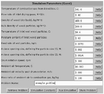
Figure 4.1: Input screen for RDS simulation.
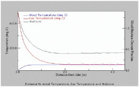
Figure 4.2: Output graph for RDS simulation.
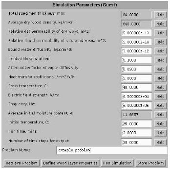
Figure 4.3: Input screen for RFP simulation
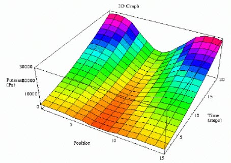
Figure 4.4: Output graph for RFP simulation.
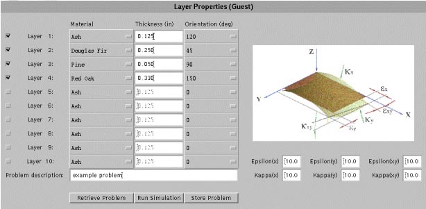
Figure 4.5: Input screen for CMA simulation.
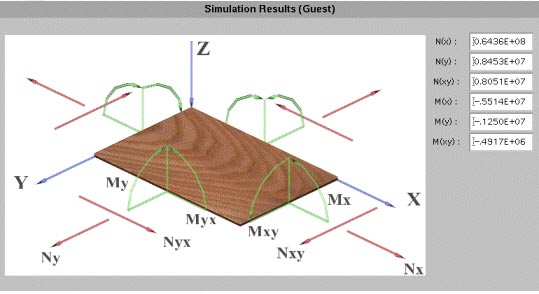
Figure 4.6: Example output for CMA simulation
Figure 4.5 shows the input screen for the CMA simulation. Each row of input data represents a layer of the wood composite. The user can add layers to the composite by clicking on the leftmost checkbox for that layer. Currently, a composite can have at most ten layers. For each layer, the user can select from a menu of materials, including several wood species and synthetic materials. The material properties are predefined. Thickness and fiber orientation may be specified for each layer. The user can enter values for various forces acting on the composite by referring to the image displayed within the applet. Clicking on "Run Simulation" executes the FORTRAN code. An example of the output produced is shown inFigure 4.6.
4.3 WBCSim Software Architecture
The software architecture for WBCSim uses a three-tier model. The tiers correspond to (1) the legacy simulations and various visualization and optimization tools, perhaps running on remote computers; (2) the user interface; and (3) the middleware that coordinates requests from the user to the legacy simulations and tools, and the resulting output. These three tiers are referred to as the developer layer, the client layer, and the server layer, respectively, as shown in Figure 4.7. WBCSim supports legacy programs written in any programming language. The only restriction is that the program must take input parameters from the command-line, one or more input files, or the standard input stream. In particular, WBCSim supports the three FORTRAN 77 simulation codes described in Section 3.
4.3.1 Developer Layer
The developer layer consists primarily of the legacy programs on which WBCSim is based. The server layer expects a program in the developer layer to communicate its data (input and output) in a certain format. Thus, legacy programs are "wrapped" with custom scripts. The scripts are written in Perl, and each legacy program must have its own wrapper script. The script receives input parameters from the server, and converts those parameters as appropriate for that legacy program. The legacy program is executed with these parameters fed to its standard input stream. The program's input may direct it to load appropriate input files. When the legacy program terminates, the wrapper script packages the program's output to create an HTML page, and passes the URL of this page to the server. The developer layer also includes tools to help developers get more from their simulations. In WBCSim this concept is implemented by integrating the legacy programs with an optimization tool and various visualization tools. The optimization tool provided with WBCSim is the Design Optimization Tool (DOT) [90].
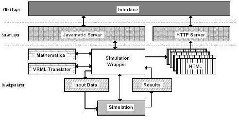
Figure 4.7: WBCSim architecture overview
DOT allows the user to provide ranges, as opposed to fixed values, for the input parameters and get a solution that either maximizes or minimizes a given output value. DOT is a sophisticated engineering optimization subroutine incorporated into WBCSim. WBCSim examples use two visualization tools: Mathematica [97] and VRML [3]. Mathematica is used to generate static three dimensional graphs of the simulation output. The output is also translated to VRML. With a VRML viewer, the resulting graphs can be viewed from various directions in the three dimensional viewspace. In principle, developers can add custom filters to convert a program's output to a useful form for any viewer of their choice. The simulations generate text output files containing raw data. The script that wraps the RFP simulation executes Mathematica to generate GIF files, and the VRML translator to generate VRML files. The HTML page generated for the results of the simulation includes links to these files.
4.3.2 Client Layer
The client layer is responsible for the user interface. It also handles communication with the server layer. This is the only layer that is visible to end-users, and typically will be the only layer running on the user's local machine. The client layer consists of the Java applets described in the previous section. After the user enters all the necessary parameters to control execution of the simulation, the client communicates these parameters along with a request to execute the corresponding program to the server layer. The server layer returns the URL for the HTML page generated from the simulation's output. The client layer directs this page to the user's HTML browser. The client layer also contains viewers for the various visualization tools found in the developer layer. WBCSim requires a VRML 2.0 viewer for the RFP model, a VRML 1.0 viewer for the CMA model, and a 3D visualization Java applet. The user is responsible for installing a VRML viewer on the local machine, but the 3D visualization applet is automatically downloaded from the HTTP server.
4.3.3 Server Layer
The server layer is the core of WBCSim as a system distinct from its legacy code simulations and associated data viewers. The server layer is responsible for managing execution of the simulations and for communicating with the user interface contained in the client layer. The main part of the server layer is the Javamatic server [78]. The Javamatic server is written in the Java programming language. The Javamatic server can direct execution of multiple simulations and accept multiple requests from clients concurrently. The results from the simulations are communicated to the clients using an HTTP server.
For security reasons, Java applets that have been downloaded from a network are not allowed to read, write, or execute files on the client's (local) file system. Since WBCSim takes input data from users via Java applets, this means that such applets must forward requests to execute the legacy application through the WBCSim server for processing. The server processes these requests and returns the results of the transaction to the client.
WBCSim uses the Java Socket class to communicate between the client and the server. Each time a user issues a command through a Java applet (e.g., he/she clicks on the "Run Simulation" button), a new client request is sent to the Javamatic server. The Javamatic server then goes through the following steps:
|
4.4 Directory Structure of WBCSim
WBCSim simulations can be accessed from http://wbc.forprod.vt.edu/pse/. All source and data files required for running WBC simulations are placed in the WBCSim home directory. The directory structure of WBCSim is shown in Figure 4.8.

Figure 4.8: Directory structure of WBCSim
A brief description of the contents of each directory in WBCSim is as follows:
|
4.5 Simulation Scenario
WBCSim incorporates the legacy FORTRAN 77 programs that implement its models without any modifications to the code. This has the advantage that if the programmer decides to make changes in the legacy program, such as bug fixes, recompilation with new libraries or newer compilers, or implementing a different algorithm, the new program can be installed in WBCSim without additional work. Figure 4.9 shows how this is possible.
Consider the RFP simulation. A Perl script (RFP Sim Wrapper) acts as a proxy between the Javamatic server and the simulation. This script is responsible for converting data from the Javamatic server to a format the RFP simulation can recognize.
In a typical scenario, the server will execute the RFP Sim Wrapper and give it all the input parameters from the command line plus an additional argument. The input parameters come directly from the client and they are a sequence of strings derived from the user's selection.
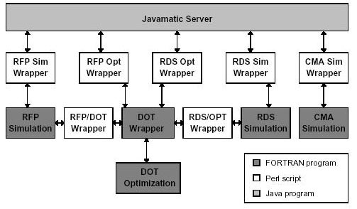
Figure 4.9: Legacy FORTRAN 77 simulation code wrappers.
The Javamatic server treats all parameters as strings regardless of whether they are boolean, numeric, or alphanumeric. The additional argument is a filename, which is accessible from the HTTP server. The RFP Sim Wrapper does not return the results to the Javamatic server, but outputs them in HTML format to that file. The Javamatic server then returns to the client the URL pointing to that file.
When executed, the RFP Sim Wrapper packages all the input parameters into a file and executes the RFP simulation. The parameters are recognized by position, thus all parameters must be present and have a value even if they are not visible on the interface or the user did not provide a value. The client has a list of default values for all the parameters that are not visible on the interface and so it fills the blanks before sending the parameters.
The RFP simulation has its own text-based user interface and requires input from the standard input stream (e.g., keyboard). The RFP Sim Wrapper takes control of the standard input stream of the RFP simulation and generates the appropriate keystrokes to read the input file and generate the results. It does this by generating a new file with all the appropriate commands and redirecting that file at the command-line when it executes the simulation. This is a temporary file and is deleted when the simulation completes execution.
While the simulation executes, RFP Sim Wrapper takes control of the standard output stream of the simulation and listens for specific string patterns. These string patterns indicate major milestones in the execution of the simulation (i.e., successful completion of a simulation step or the computation of an intermediate value). RFP Sim Wrapper then generates a message and outputs it to the standard error stream. The Javamatic server captures that message and propagates it to the client. Eventually the message gets to the user. The standard error stream is used, instead of the standard output stream, because Java buffers the standard output stream and makes it available only after the process terminates. In contrast, the contents of the standard error stream are sent continuously to the parent of this process. Arbitrary network delays can cause a group of messages to be delivered simultaneously, even though they were generated at different times. The client always displays the latest message and discards any old messages.
When the simulation terminates, the wrapper takes the results and creates a file, in HTML format, with the filename given by the server. This file contains a list of links that point to the results in various formats. The RFP Sim Wrapper then runs Mathematica to read the results, which are in textual format, and generates a 3D Plot, which is a Mathematica internal data structure. RFP Sim Wrapper then calls the appropriate Mathematica function to output the 3D Plot to a file in encapsulated postscript format. It also calls the VRML translator to generate a VRML wireframe representation of the results. RFP Sim Wrapper executes a series of filters to convert the results to GIF images. RFP Sim Wrapper also creates text and HTML-table versions of the results. All these different views are stored in individual files on the server. An archive tool manages the files from different simulation runs.
A benefit of using the simulation code in a PSE environment is that other software tools, such as the DOT optimizer, can be used to provide more functionality to the end-user. The user can provide a range instead of a fixed value for any of the input parameters and specify which component in the output to maximize or minimize. RFP Opt Wrapper, a Perl script, receives the input parameters from the server plus the variables to optimize and a filename. The wrapper then packages all the input parameters in a file and executes DOT Wrapper, which is a FORTRAN 90 program. RFP Opt Wrapper gives DOT Wrapper the filename that contains the data plus the name of the program to call every time the optimizer asks for an evaluation of the objective function. RFP/DOT Wrapper executes the RFP simulation once and returns the objective function value. When the optimizer finishes, DOT Wrapper returns the optimal parameter values and objective function value to RFP Opt Wrapper. RFP Opt Wrapper then executes the RFP simulation one more time and packages the results in the same format that RFP Sim Wrapper uses. The advantage is that neither the simulation code nor the optimization code needs to be changed. To add a new optimizer with a different optimization algorithm, the only thing that needs to be done is to modify the wrapper script DOT Wrapper. The simulation code and RFP/DOT Wrapper remain the same.
4.6 Visualization
VRML was chosen as the primary viewing environment for simulation output. Our approach is to convert output generated by FORTRAN into a VRML description so that the output of the simulations can be visualized interactively. A custom-built translator provides greater control over the description of 3D models that third-party translators cannot provide. VRML was chosen for the following reasons: (1) VRML is a recognized standard for visualizing 3D worlds. (2) VRML viewers are available for a wide variety of platforms, and most of them are easy to use. (3) VRML syntax is simple, and VRML code can be easily generated by programs [70].
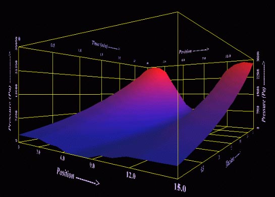
Figure 4.10: Pressure graph showing the variation of pressure with increasing distance from the laminate surface and with time (the receding axis).
VRML models were generated for the radio-frequency pressing model and the composite material analysis model.
Radio-frequency pressing model: The output data generated by RFP is a matrix of numbers where each number represents the value of a dependent variable with respect to two independent variables. Since this is a two-dimensional data matrix, it is conveniently modeled as a VRML ElevationGrid as shown in Figure 4.10. The dependent variable here is "Pressure" (y axis), which is now represented by variations in the height of the elevation grid, and the independent variables are "Position" (x axis) and "Time" (z axis). Each element in the matrix becomes a colored point on the grid, and the color is smoothly varied between the grid points.
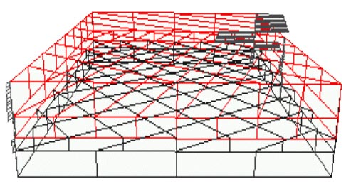
Figure 4.11: Wireframe model of a composite showing failed layers (red) and active layers (black), and the orientation of fibers in each layer. In this figure, the second layer has failed. The horizontal protrusions are proportional in length to the magnitude of forces being applied to the layers at the time of failure. The direction of the protrusions is unimportant.
WBCSim also provides a variant of this model where elements in the matrix are represented by squares rather than points, and a different color is assigned to each square, resulting in a checkered elevation grid.
To ensure that the top and bottom views of the elevation grid are able to indicate the true height of the grid points, each grid point is colored based on its height, with blue representing the lowest point on the grid, and red the highest. All other grid points are colored by linearly interpolating between blue and red color values.
Composite material analysis model: In this simulation, the output contains information about the forces being applied on various layers of a composite when one or more of the layers fail due to an applied load. The composites are tested for strength based on their material property, thickness of layers, and orientation of the fibers in each layer. Material properties may be selected from a menu of various wood species. Five testing methods have been implemented: analysis, design, tensile strength, bending strength, and shear strength. In the analysis method the program calculates the deformed shape of a multi-layered composite laminate (e.g., plywood) caused by user-defined loads and moments. In the design method the program calculates the applicable loads and moments which cause a user-defined deformation of the multi-layered composite. The other three methods calculate the magnitude of the load (tensile, bending, or shear) which causes the multi-layer composite laminate to fail. In the analysis and design methods, one or more layers may or may not fail, whereas in the other three methods, the simulation continues until all the layers fail. It is the job of the VRML translator to decide which layers have failed by looking at the FORTRAN-generated output files. Each time a layer fails, a new VRML model is generated containing information about the forces on each layer at that instant. Failed layers are displayed in red, whereas active layers are displayed in black, as shown in Figure 4.11.
Chapter 5
Conclusions
This thesis presented two problem solving environments for vastly different application domains. Both the PSEs addressed the issue of integrating visualization with computation, and showed how visualization can increase their power and utility, allowing the researcher to think in terms of the overall task of solving a problem, not just viewing the results of the computation.
As a PSE for aircraft design, VizCraft provides a framework that allows the designer to visualize databases of HSCT designs using a system of parallel coordinates. The implementation of parallel coordinates into VizCraft allows the user to visually manipulate the design space while searching for patterns, and to eliminate portions of the design space from consideration by carefully selecting regions of interest. However, an intuitive feel for this application of parallel coordinates can only be realized with some practice, just as an intuitive feel for Cartesian representations is developed through usage and practice. While implementing the parallel coordinates system in VizCraft, special consideration was given to two aspects: user interactivity for allowing interactive data exploration, and modularity, which is necessary for adapting the system in the future to the needs of different applications, not just those specific to HSCT design. The parallel coordinates module in VizCraft has been used to display multidimensional data sets for other application areas as well, provided the data file supplied to it is in the required format.
VizCraft is a classic example of an application where complex operations are abstracted into a coherent form at the level of the user interface. By incorporating both computation and visualization facilities, and making them accessible through a high-level user interface, VizCraft has helped HSCT designers be more productive in a number of ways. The interface has streamlined the practice of exploring the effect of design variable combinations on aircraft performance for regions of the design space that have not previously been investigated. Where the designer originally had to manually change design variables in a file, run the analysis code, and then observe the results in a separate plotting package, VizCraft is able to perform these operations with a few clicks of a button. The data mining capabilities of VizCraft have also proved beneficial when large databases of HSCT performance data are available. Through the use of colored driving variables and the brushing techniques, designers were able to visually correlate different design variable combinations/patterns that resulted in either very good or very bad aircraft performance.
WBCSim provides a Web-based graphical user interface to legacy FORTRAN simulation codes in the wood-based composites domain. Providing a Web-based front end has the following benefits:
|
In short, WBCSim provides an integrated set of high-level facilities for solving problems in the wood-based composites domain. It allows users to define, record, and modify problems, and to visualize and analyze simulation results, which is the very essence of a PSE.
The original motivation for creating WBCSim was the more obvious effects of improved usability provided by the graphical user interface and Web-based access. These effects in themselves would be enough to make WBCSim a success for the research group that depends on these WBC models. However, there are more significant effects of WBCSim on the group's productivity, which were not so clearly predictable in advance. These effects are related to the synergistic nature of combining the models, an optimizer tool, and a visualization tool. The resulting integrated package immediately led to greater use of the simulation models by the researchers. Not only did they use the models more, but they used them to examine the design space in new ways. This is borne out by the fact that the researchers started to use parameter settings that caused the simulations to fail, that is, they uncovered new bugs in the simulation codes. Once these bugs were corrected, the researchers were able to continue more extensive use of the models.
It is likely that this integration effect will arise in many application domains. In general, an increased ability to integrate simulation, optimization, and analysis tools will allow researchers to get more out of their tools as they find new ways to make use of them.
5.1 Directions for Future Work
The current implementation of VizCraft consists of two parts: a graphical user interface to the HSCT code, and a visualization module. While this is a complete application in itself, the current implementation is missing two important features. Possibilities include (1) remote access via the WWW, and (2) integrating optimization capabilities.
The World Wide Web offers opportunities for making visualization techniques available to the general public. The necessary components to access the Internet and the WWW are already available to the public and widespread. Java offers the required functionality to design the user interface and communication between a client and a server. Providing a Web-based environment to VizCraft will offer several benefits that WBCSim already provides: it will enable a wider class of users to access it away from their workplaces, and from a variety of platforms. Users of VizCraft will not need to worry about software installation issues at the client, anybody with a Java-enabled Web browser and an Internet connection will be able to execute VizCraft.
VizCraft does not incorporate any of the optimization tools currently being used for HSCT design. Integrating an optimizer like the Design Optimization Tools (DOT) [90] package with VizCraft can greatly increase the power and utility of VizCraft. DOT is currently being used with only the HSCT design evaluation. The VisualDOC design optimization software [37, 91], in addition, provides a graphical user interface to DOT, and may be a good candidate for integrating with VizCraft in the future. With the integration of an optimizer, users could potentially provide an acceptable range for any of the design parameters, specify which of the output values to minimize or maximize, and observe, and possibly alter, the optimization run as it is being executed.